In this article, we will see how to freeze a row in Excel using 5 Easy Steps. If you work on Microsoft Excel, then sometimes you might have faced a situation where you need to keep an area of a worksheet visible while you scroll to another area of the worksheet. This can be easily achieved from the View tab in Excel, where you can Freeze Panes to lock specific rows and columns in place, or you can Split panes to create separate windows of the same worksheet. We will see the steps in detail with the help of an example in below section. More on official website.

How to Freeze a Row in Excel Using 5 Easy Steps

Also Read: NtCreateFile failed: 0xc0000034 STATUS_OBJECT_NAME_NOT_FOUND

Step 1: Prerequisites

a) You should have a running Windows System.

b) You should have Microsoft Excel installed in your System.

c) You should have access to edit the Excel file.

 

Step 2: Select Row

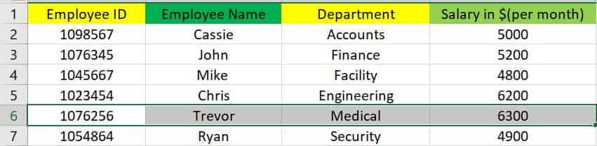
If you have an excel worksheet like below where you want to freeze the rows from 1 to 5 and make it visible while you scroll to another area of the worksheet then you need to select row 6 and click on View tab from the top of the excel.

 

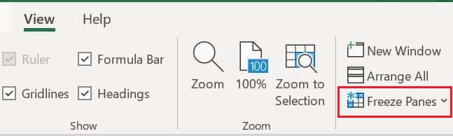
Step 3: Open View Tab

Once you open the View tab, you need to select Freeze Panes option and click on drop down arrow as shown below.

 

Step 4: Select Freeze Panes

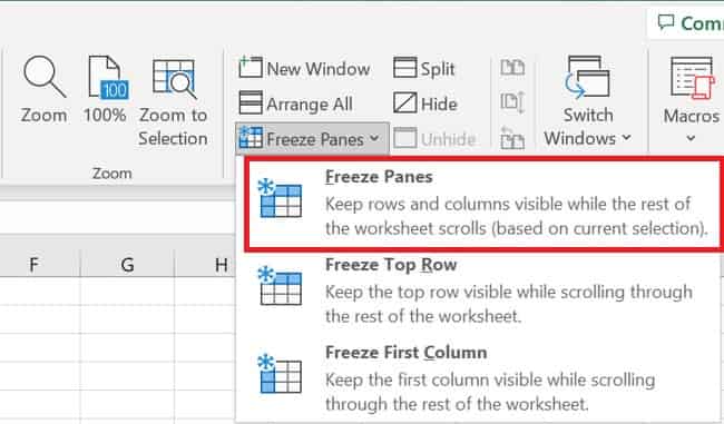
In the drop down, you will see three options - Freeze Panes, Freeze Top Row and Freeze Top Column. If you are looking to make the top row visible while scrolling through the rest of the worksheet then select Freeze Top Row and if you are looking make the first column visible while scrolling through the rest of the worksheet then select Freeze First Column.

But in our case we are looking to make rows and columns visible while scrolling through the rest of the worksheet based on our current selection so we need to select first option in the drop down i.e Freeze Panes as you can see below.

 

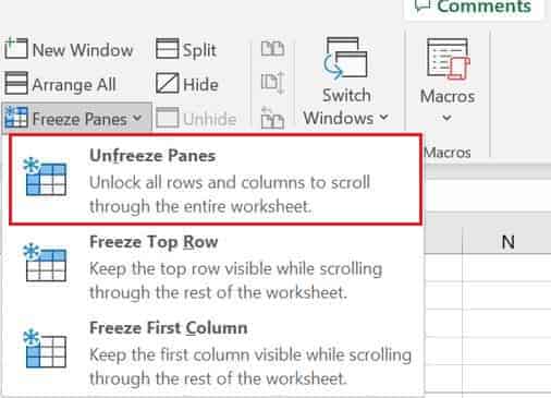
Step 5: Select Unfreeze Panes

Similarly, if you are looking to unfreeze the freeze rows and columns, then you need to again select the row and click on View tab from where you can unfreeze the rows and column by clicking on Unfreeze Panes option in the drop down as shown below.